Balancing Basics

Download Balancing Basics (PDF)

Comdronic Ltd would like to extend gratitude to the following companies for the photographic images that support this document.

Crane Fluid Systems www.cranefs.com
Oventrop UK Ltd www.oventrop.com

A basic discussion of the processes involved to establish the flow of water through valves which, in turn, will lead to the balancing of water flows in the various parts of a water based system.

Balancing basics is intended to be used by engineers and technicians who are not specifically trained as commissioning engineers. It can also be used as a reference for those training to become commissioning engineers.

The flow of water in a system with multiple branches and terminals might at first glance seem mystifying, however, a basic knowledge of the physics involved will help to clarify the process.

The type of system we are interested in for flow balancing is a closed loop system such as a heating system or chilled water system.

Those of us with central heating systems at home have all endeavoured to get the balance right in the system by simply adjusting each radiator until it feels ‘about right’ This process is ok if we have enough time, however, if the system is large, such as a commercial heating system then the process has to be formalised to ensure correct building comfort.

If we are to ensure that the space is heated or cooled by the correct amount we have to make sure that the flowrate of water to the space is in keeping with the requirements set out by the design engineer. Each space will have been analysed for heat loss/gain and a heating/cooling load in kW (kilowatts) determined.

In order to transport the kW to the space we use water either heated or cooled. The designer will normally convert the kW value into flow rate using the formula:

Mass flow rate = Emitter output (kW) / Specific heat capacity for water X ∆t (Deg C).

For heating the temp change (∆t) in the emitter is usually 11 Degrees
For cooling the temp change (∆t) in the emitter is usually 6 Degrees

The specific heat capacity of water is 4.187 kj/kgC

Because the ∆t in cooling is less than that in heating we can see that for each kW delivered to the space we will need more water if it is cooling.

Do not let any of the above cause you concern because the designer will have already carried out the calculation for flow rates and it is this that we are interested in.

The basic building block for the commissioning engineer is the balancing valve. This is a generic term for a variety of valves used for balancing systems. There are 4 main varieties of traditional device as described below.

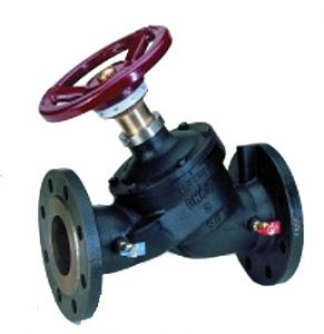
Double Regulating Valves (DRV)

For flow regulation only.

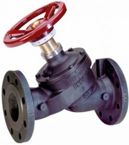
Typically this valve is a Y pattern globe valve arranged in this way to present the smallest pressure loss to the system when fully open. Adjustment of this valve will add resistance to the system and hence reduce the flow. The description DOUBLE regulating means that it has a feature whereby you can set the position that the valve is to operate at in such a way that you can still close the valve for maintenance purposes.

Flow Measurement Devices & Valves (FMD / FMV)

For flow measurement with or without isolation facility.

These devices are usually fixed orifice devices. More recently there has been more venturi devices appearing on the market (Mostly from US). A fixed orifice is the simplest device that we can use for measurement. The fixed orifice can be used on its own or with an isolating valve fitted downstream to provide isolation. Installed on their own these devices can give the most accurate results. When using electronic manometry to display the flow through this product the Maker, model and size of the unit must be entered into the meter. (See section ‘Taking readings’)

Double Regulating Valves combined with Flow Measurement Devices (FODRV)

For regulation and flow measurement combined in one valve unit based on the Fixed Orifice principle.

This combined assembly traditionally was assembled from a double regulating valve and fixed orifice device. More commonly nowadays the orifice is fitted directly into the body of the valve.

When made up of a regulating valve and separate orifice the unit is often referred to as a ‘Commissioning set’.

When using electronic manometry to display the flow through this product the Maker, model and size of the unit must be entered into the meter.

(See section ‘Taking readings’).

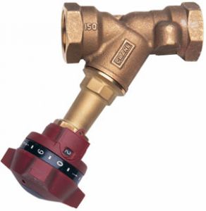
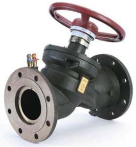
Double Regulating Valves with integral Flow Measurement facility (VODRV)

For regulation and flow measurement combined in one valve unit based on the variable orifice principle.

Shown in the photo is a cast iron VODRV which allows the measurement of the flow across the entire valve. There is no fixed orifice fitted to this valve – the signal measured on an electronic manometer relates to the loss across the whole valve.

When using electronic manometry to display the flow through this product the Maker, model and size of the unit must be entered into the meter. (See section ‘Taking readings’).

Because the signal being measured on this valve relates to the loss across the entire valve the size of the signal depends on the position of the handwheel. This process will be dealt with in some detail later and really only affects those working on systems overseas. The use of this type of valve is popular in Europe and Ex Russian states.

Before any readings can be taken it is important to identify the type of valve or orifice device being used. The section above describes each type of device but when approaching a job on-site it might not be so obvious as to the type of valve in use.

The first job is to identify which valves are for measuring and which are simply installed for regulating.

Rule 1 is to check for testpoints installed on the valve. If there are no testpoints then the valve is a simple regulating valve which will have been installed to regulate flow. The measurement of flow will have to take place elsewhere. Typically in these instances a fixed orifice might be installed for measurement purposes. If the regulating valve is installed on the return side of a circuit then the orifice might be installed on the flow side. (This is not always the case but is usual).

Regulating Valve

Fixed Orifice

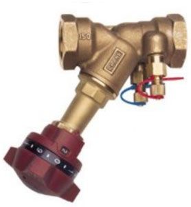
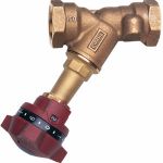
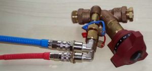
If the valve is fitted with testpoints then a bit more care is required. The first valve shown below has testpoints fitted which are a significant distance apart when measuring along the axis of the valve.

This indicates that the differential pressure will be measured across the entire valve. If this is the case then the size of the orifice will change when the valve is operated. This valve is therefore aVariable Orifice Double regulating valve  (VODRV).

If the valve is fitted with testpoints that are very close together when measured along the axis of the pipe then the valve is likely to be a Fixed Orifice Double Regulating Valve (FODRV).

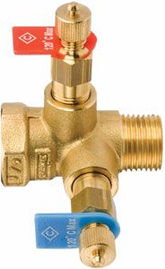
Important note: Some European manufacturers fit testpoints on the stem area of the valve body.

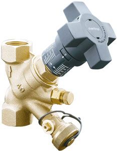
The Oventrop example here shows a combined testpoint and drain unit very close to another testpoint. This valve is a variable valve. The testpoint nearest to the centre of the valve is ported downstream of the valve seat.

If in doubt get the information from the manufacturer.

For all discussions relating to measurement using valves as described above we will only consider the use of electronic manometers such as Comdronic AC6, Crane and Hattersley ProComm, Cimdronic AC6, Frese AC6, MMA AC6 and LRI 8170.

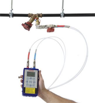
The principle behind the measurement of flow through a balancing valve is the way in which we exploit the pressure loss created across the orifice or valve when water flows through it. We know that every device inserted into the system will create a small amount of resistance to flow. The resistance to flow will create a situation where the pressure on the inlet side of the valve will be very slightly higher than the outlet side of the valve. This difference in pressure is called the DIFFERENTIAL pressure or SIGNAL.

The design and manufacture of the balancing valves is carried out to strict limits of tolerance so that the signal read across one valve of a type is the same as another. Small errors do exist but these keep the overall measurement tolerance to a very small level.

Using an electronic commissioning meter the following calculations are carried out automatically but the mathematics is included for those wishing to see how we arrive at the flow rate.

The only reading we take with the electronic manometer is the differential pressure (dP) – When we have taken the reading we have to equate this to the balancing valve design figures so that we can establish the flow through the valve.

Each valve is given a value which links the dP with the flow rate. This value is the Kvs value. The equation which we commonly use in the UK is:

Flow ‘Q’ = [Kvs X √dP] / 36 Flow is litres/second

dP is KiloPascals (kPa) Note: 100 kPa = 1 Bar = 10 metres head This formula is very simple to use.

1. Take the reading from the balancing valve or orifice device and find the square root of the value.
2. Establish the Kvs value for the balancing valve or orifice device (From manufacturer chart.
3. Multiply 1 and 2 above and divide the answer by 36
4. The answer is now the flow rate.

As an example let us say that the dP reading is 5.2 kPa across an orifice device which has a Kvs of 2.2 – the calculation is as follows:

Flow Q = [2.2 X √5.2] / 36

= [2.2 X 2.28] / 36 = 0.139 L/S

Now- if you know the flowrate that you are seeking and want to calculate the dP value that you have to adjust the valve to achieve we need to re-arrange the formula.

dP = [36Q / Kvs]²

Simply multiply the desired flow rate by 36 then divide by the Kvs and finally square the answer.

So- if we are looking to adjust the valve to achieve 0.139 L/S our calculation is as follows:

dP = [36 X 0.139 / 2.2]² = 5.2 kPa

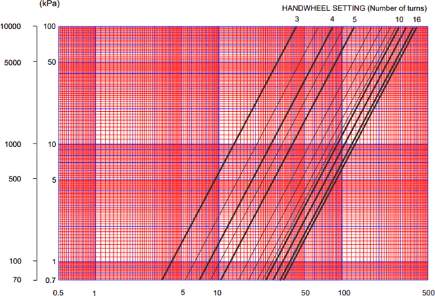
In order to simplify the process of deriving the flow from the measured differential pressure the manufacturers publish graphs for each of the valves as shown below.

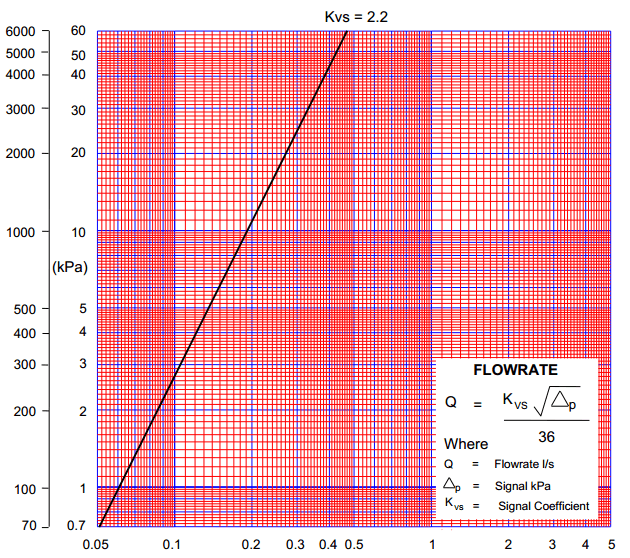
Graph showing performance of valve with Kvs 2.2

To derive flowrate from graph simply take the differential pressure reading in kPa and find this value on the vertical (Y) axis – Read across and from the point where the lines cross read down to find the flow.

Note: the graphs are log/log graphs so care must be taken to derive the correct flow.

If you are using any of the electronic meters mentioned above all you have to do is enter the correct measuring device or balancing valve into the meter using SELECT VALVE option. The information entered is Maker, type, model and size.
When you return to the display screen the type of valve will be displayed on the scroll bar at the bottom of the screen.

The dp can be taken from the valve and the flow is automatically calculated and displayed. The calculations shown above are all taken care of by the meter.

Fixed orifice devices

1. Identify the maker, type, model and size of the valve being measured.
   (For our purposes we will assume it is a Crane fixed orifice type D931 size 15mm.)
2. Select the correct connection fittings provided with the electronic meter. For the Crane valve we need the angle insertion probes. (These are often referred to as ‘Binder’ adaptors)
   
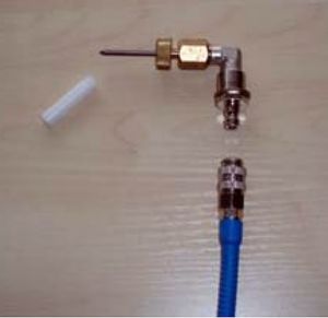
3. Remove white plastic protectors and snap the connectors onto the red and blue tagged nylon connection tubes. It is possible to connect to either end of the tube – it would be normal to connect it to the end opposite that with the ball valve fitted. (The end you choose is personal preference)
4. Connect the other end of the two connection tubes to the electronic meter.
5. Ensure that the small bypass valve on the side of the meter is OPEN. And the two ball valves on the connection tubes are closed.
6. The insertion probes can now be inserted into the fitting (testpoint) on the Crane D931 valve. It is advisable to wet the probe first as this has to push its way through a rubber seal in the testpoint. This can be difficult especially when the testpoint is new.
   
7. Open both ball valves on the connection tubes. If there is a flow through the Crane balancing valve there will be a differential pressure across the valve which will force water through the red connection tube, through the meter and back to the balancing valve via the blue connection tube. This process known as purging can only happen when the small bypass valve is open.
   When the flow through the balancing valve is high the dP will be large and will purge the tubes quickly. When the flow is low then the process could take some time (1-2 minutes).The nylon tubes are supplied in clear nylon to allow you to see the air bubbles being purged. Do not leave the unit purging for more than the necessary time as this can make the internal temperature of the unit change dramatically, particularly on heating systems. The unit has temperature compensation built-in but changes in temp take some time to settle.
8. Close the two ball valves on the unit. Switch the unit on by pressing any button. When the unit starts it will ‘boot-up’ to a display screen which is defaulted to show FLOW and PRESSURE. Look at the pressure reading to establish if the unit has settled following the purge process. Press the zero button. The display should now display zero and be stable on this reading. Re-zero the unit if necessary. The unit is now ready to read from the balancing valve.
9. Open the two ball valves on the connecting tubes and then close the small bypass valve on the unit. The pressure reading should now be showing.
10. To display the flow reading it is necessary to enter the valve into the unit. Press the menu button and use the right arrow button to change menus until MAIN menu is displayed. The first item in this menu is SELECT VALVE press the tick ( S ) button.
11. Use right arrow button to select maker (Crane in this case) – when Crane is visible use down arrow to move in the menu to the valve type – this is FIXED in our example. Use down arrow to move to menu item valve type – this is D931 in our example so you will have to use the right arrow button to find the valve. When found use the down arrow to move to the size option. The first size is 15mm. At this point you can look at the complete selection. It should be Crane-Fixed-D931-15mm. At this point press the tick button to select.
12. The screen display will now return to the PRESSURE and FLOW screen. The flow will now be displayed.

Note: because a period of time has elapsed it may be necessary to re-zero the unit. To do this make sure that you open the small bypass valve first followed by closing the ball valves. Re-zero at this point then open the ball valves followed by closure of the bypass valve. You should now be reading flow and pressure.

Please remember to open the small bypass valve each time you zero the unit or move the unit from one balancing valve to another. The bypass valve in the open position provides additional protection to the sensor from harmful overpressures which can be present when the unit is disconnected and re-connected.

Variable Orifice Devices (VODRV)

Why use this procedure? This procedure is for setting the handwheel on a VODRV such that the desired flowrate is achieved without having to refer to manufacturer’s multi line graphs.

It is important to note that the KVs value of the valve changes as the handwheel is operated. Therefore the flow reading cannot be taken from the AC6 until the handwheel position has been entered into the meter.

How do I know if the valve is VODRV or a fixed device? If there is any doubt about whether a variable orifice valve is being measured then simply take a differential pressure (dp) reading when the valve is fully open and then close the handwheel by a couple of turns. Without changing anything on the meter if the differential reading appears to go up and the flow appears to go up then the valve is a variable orifice valve (VODRV)

If the same procedure is used and the dp and flow go DOWN then the valve is a FIXED orifice device.

Information that you will need to have available.

1. The MAKE, MODEL, TYPE AND SIZE of the valve being measured
2. The desired flowrate through the valve.

Procedure for setting the valve.

1. Select the correct valve and size from the database using MAIN MENU- SELECT VALVE-MAKER- MODEL- SIZE
   Return to the display screen using the X button or return button (bottom left) – The correct valve should now be scrolling across the bottom of the screen.
2. Enter the desired flowrate for the valve using MAIN MENU- DESIGN FLOW Return to the display screen.
3. Change the display menu to MULTIDISPLAY in the DISPLAY menu

You should now see a display with a lot of information. On the right hand side there is the DP and the FLOW readings. On the left side in a small box there is the PERCENTAGE OF DESIGN FLOW.

With the balancing valve connected and set in the fully open position the flow reading on the meter will be correct because the meter is automatically set to the fully open position when it was selected. The handwheel position is shown at the top of the small valve schematic image on the left of the screen.

Assuming that when the valve is fully open there is a surplus of flow then the PERCENTAGE OF DESIGN FLOW box will show a figure greater that 100%
If the figure is less that 100% then the balancing valve will have to be left fully open.

Because the adjustment of a balancing valve can have a varied effect on the flowrate due to the unknown authority the valve has over the circuit, the process of adjustment involves an iterative process and some careful judgement.

Let us assume that the flow percentage in the lower box is 120% then we know we must close the valve slightly to reduce the flow. If we have a valve that has 8 full turns to the handwheel then we can attempt to set the valve to say, position 7. We must now adjust the handwheel position in the meter also the position 7 ( Using the UP arrow) At this point the flowrate reading will now reflect the flow through the valve at handwheel position 7. Again, because we are unaware of the authority of the valve over the circuit the flow might either be higher than design or perhaps lower than design.

If the flow is higher than design then the balancing valve must be closed a little more and the new handwheel position entered into the meter. Keep using this method until the percentage of flow through the valve is at 100% of design.

In order to achieve a quick adjustment it might be better in practice to ‘over-adjust’ the valve so that the user can assess the effect of the valve authority over the circuit. With practice the user should be able to set the valve correctly with perhaps only 3 or 4 adjustments.

This process may seem involved but it is a lot simpler than trying to use the graphs provided by the manufacturers.

Please note: the handwheel setting shown in the percentage box adjacent to the left arrow symbol is the setting that would be correct if the differential pressure was constant when the valve is adjusted. This setting should not be used unless differential pressure controllers are present in the circuit.

What do I do if I need to restart this procedure?

If the process of setting the valve has not gone according to plan then we can reset the meter and balancing valve to the start position.

1. Use the UP arrow key which will prompt for a handwheel setting. At the top of the screen the max and min handwheel positions are shown. Set to the Max POSITION.
2. Adjust the balancing valve to the fully open position.

Check on the MULTIDISPLAY screen that the handwheel position shown above the schematic is the correct fully open value.

Now start the setting procedure again.

Remember that each time you move from one balancing valve to another the meter and the valve have to be set for the fully open position before starting the procedure.

Now that we are able to establish the flow rate through a balancing valve the next step is to understand the process of balancing.

In the UK we use a system of balancing called ‘Proportional Balancing’. The reason for this name will become apparent later!

The balancing process described here is simply a guide to the principle of proportional balancing. It is important to point out that the pre-commissioning checks need to be made, these however are not the subject of this paper. The pre-commissioning checks would include but would not be limited to:

1. Installation check to manufacturer’s requirement.
2. Inclusion of correct venting and draining
3. Inclusion of correct strainers
4. Correct installation of measuring/balancing valves with respect to pipe size/type and the clear lengths of upstream/downstream pipe
5. Checks on the correct chemical cleaning
6. Checks on the correct water treatment
7. Checks on glycol content if used.
8. Checks on pump motor conditions

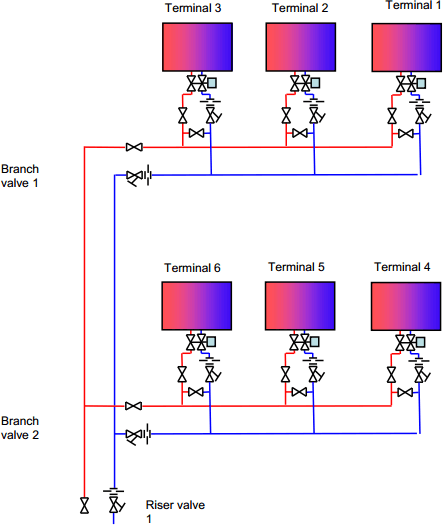
Referring to the idealised system above we will assume that the pump is located at the base of the riser and each of the terminals is designed to have the same flow rate. We will assume that the pump has been sized to give a small percentage extra flow (This is quite common although nowadays variable speed pumps allow for this).

Assume that each terminal is to have 0.1 l/s flow and the valves have a Kvs value of 2.2

We have 6 terminals therefore we have a requirement for 0.6 l/s flow.

If we are using an electronic commissioning meter the process will be as follows:

1. Ensure that all balancing valves and control valves are fully open.
2. We have to establish which terminal is getting the least flow. Generally the terminal furthest from the pump is likely to have the greatest resistance to flow because of the length of pipe connecting it to the pump. This is not always the case so it is wise to carry out a quick check by measuring the flow at each of the likely terminals. In our example we would perhaps check terminal 1, 2 and 4.
3. The terminal with the lowest flow is the INDEX circuit. Note: if all the terminal balancing valves are the same then it is a simple process to check which is the index circuit – the circuit with the lowest dP showing when connected to the meter.
4. We will assume that terminal 1 is the index.
5. Take a flow reading at terminal 1 – this is likely to be something other than 0.1 l/s -for this example we will say the flow is 0.096 l/s which is 96% of our requirement. The important point here is that we are in ‘underflow’ and adjusting the balancing valve will only reduce the flow. Do not be concerned with this, simply record the percentage of flow (i.e. 96%)
6. Take a reading at terminal 2 – this is nearer the pump so the flow will be slightly higher than terminal 1 – say 0.098 l/s. We must now make a small adjustment to the balancing valve so that the percentages are the same i.e. 96%. We can now say that the terminals 1 and 2 are balanced even though they are still in underflow.
7. Take a reading at terminal 3 – again, this is nearer the pump and perhaps the percentage of flow is 102%. We must again adjust the balancing valve until we achieve the same percentage through terminals 1, 2 and 3.
   Note: We must remember that because we are making adjustments to balancing valves we are forcing water to go elsewhere – some of this water will go through the previously set terminals so a quick check on terminal 2 will establish if there has been any increase in the percentage. If the flow has increased then make the necessary adjustment to terminal 3 so that the percentages are all the same.
   Remember that a quick check on the previous valve will reveal the flow percentage through all of the previously balanced terminals because they are balanced.
8. We now have a branch where all three terminals are balanced and the percentage of flow is 96% (assuming it has not changed when making the adjustments)
9. Take a reading at terminal 4 which is much nearer the pump and will therefore have a higher percentage of flow – say 114% Record this figure.
10. Continue with the balancing process on this branch in exactly the same way as the previous branch.
11. When you have completed this the terminals will be balanced at ‘say’ 114%
12. We must remember the effect of making adjustments to balancing valves will affect the flow elsewhere in the system, as such, the first branch may have increased.
13. Take reading on branch valve 1 which might have increased to 98%. We now have a situation where the flow in the top branch is 98% and the lower branch 114%
14. With the meter set on branch valve 2 adjust the valve until this branch is the same percentage as the first branch. We have already discussed the fact that by adjusting a valve the water will flow elsewhere and it is for this reason that checks of the flow in branch 1 need to be made. As the flow reduces in branch 2 when adjusting the valve the flow will increase in branch 1. A second meter or perhaps a manometer set on branch 1 would be useful in this situation.
15. The adjustment is made to equalise the percentage flow and in our example this might be 106%
16. All terminals and branches are now balanced at 106%. The final measurement and adjustment being made to riser valve 1 which should show that the flow is 106%. Make the adjustment to 100%.

By adjusting just the one riser valve all terminals are affected by the same PROPORTION!

The process described above is very simplistic but it gives details of the basic requirements of proportional balancing. Commercial systems are normally far more extensive than the system described but the process of creating balanced groups of valves such as branches before balancing the branches with each other can be extended to balancing multiples of branches or even multiples of risers.

We have discussed the principle of ‘percentage’ of design flow where the actual flow is related to the design flow. This process is made very easy with any of the above electronic commissioning meters. Simply select the correct menu to enter the design flow for the valve being measured and then display this using the MULTI display. The percentage of design flow will be displayed alongside the actual flow and differential pressure. As the balancing valves are adjusted the percentage of design flow figure will change.

Using the AC6 meter will reduce the laborious task of continued reference to the flow charts or tedious calculations.

The AC6 electronic manometer is designed to facilitate measurement of systems using traditional balancing valves as shown above. Standard software within the unit also allows the display of flow associated with automatic balancing valves. The AC6 is unique in this area and coupled with its ability to store data (using optional PcomPRO software add-on) makes the unit the preferred meter for commissioning engineers.

Further reading

CIBSE Knowledge guides Commissioning code W (2010)

BSRIA guides. Commissioning water systems BG2/2010 Commissioning Specialists Association

Acknowledgements

Crane Fluid Systems

Oventrop